Inversion number: deep dive into sorting algorithms

10 Feb, 2025

An inversion in a sequence is, as defined by Wikipedia, “a pair of elements that are out of their natural order.”

If we define a sequence $A = (A_{1}, \dots, A_{n})$ , and define the increasing order as its natural order, then any pair of $(A_{i}, A_{j})$ where $i < j$ and $A_{i} > A_{j}$ is an inversion.

The number of inversions in the sequence $A$ , namely the “inversion number” $inv (A)$ is, naturally, between 0 and $\frac{n (n - 1)}{2}$ .

Today, let us explore different algorithms for calculating inversion numbers, from simple brute force approaches to the most efficient methods. Later, you’ll understand why the title mentions “sorting algorithms.”

Brute force

The most brute-force way must be emulating all pairs and checking if they match the criterion:

def brute_force(A: list[int]):
    count = 0
    for i in range(len(A)):
        for j in range(i + 1, len(A)):
            if A[i] > A[j]:  # criterion
                count += 1
    return count

The runtime complexity is $O (n^{2})$ .

Insertion sort

Another way to think about it is that the inversions are negated when we swap them, and by this means, the sequence becomes closer and closer to the expected order. This is, of course, an insertion sort. Therefore, we can calculate swaps during the insertion sort, like this:

def insertion_sort(A: list[int]):
    count = 0
    for i in range(1, len(A)):  # current element to insert
        last_val = A[i]  # store the value temporarily
        for j in range(i - 1, -1, -1):
            if last_val < A[j]:
                A[j + 1] = A[j]  # move one place to the right
                count += 1
            else:
                break
        A[j + 1] = last_val  # put to the right position
    return count

The runtime complexity is, of course, still $O (n^{2})$ .

Well, now that we’ve come to this, it seems that the answer really lies inside the “sorting.” If we want to optimize our algorithm, we probably have to rely on a more optimal sorting algorithm, e.g., merge sort, heap sort, or even counting sort.

Let us try each of them, one by one.

Merge sort

When we are doing the merge sort, we essentially cut the sequence into halves, and quarters… And then merge from the smallest chunk, to the final complete sequence (which is fully sorted). The swaps inside one chunk won’t influence the inversion numbers of chunks outside of that chunk, and vice versa. Therefore, it seems that we can still infer the inversion numbers from swaps. But how?

Say we have two halves of a sequence, namely $(A_{left}, \dots, A_{mid - 1})$ and $(A_{mid}, \dots, A_{right - 1})$ , both are sorted, and we are doing the final step of merging the two halves together to get the fully sorted sequence. Suppose we are in the middle of merging, with indices $i$ and $j$ currently, like this:

Snipaste_2026-02-06_20-01-17

If $A_{i} > A_{j}$ , then all elements right to $A_{i}$ , i.e., $(A_{i + 1}, \dots, A_{mid - 1})$ must also be greater than $A_{j}$ . Therefore, by letting $A_{j}$ be put first in the final sequence, not just one swap is performed, but $mid - i$ swaps (imagine we are inserting $A_{j}$ before $A_{i}$ , then all to the right of $A_{i}$ need to move one position to the right).

Let’s modify the merge sort to implement the count of inversions:

def merge_sort(A: list[int]):
    def merge_sort_recursive(A: list[int], left: int, right: int):
        if left + 1 >= right:
            return A, 0

        # Divide and conquer
        mid = (left + right) // 2
        A, left_count = merge_sort_recursive(A, left, mid)
        A, right_count = merge_sort_recursive(A, mid, right)

        # Merge already sorted two halves together
        merge_count = 0
        i = left
        j = mid
        B = []  # to store the sorted result
        for k in range(left, right):
            if j >= right or (i < mid and A[i] <= A[j]):
                B.append(A[i])
                i += 1
            else:
                B.append(A[j])
                j += 1
                merge_count += mid - i  # inversions
        A[left:right] = B

        return A, left_count + right_count + merge_count

    A, count = merge_sort_recursive(A, 0, len(A))
    return count

The runtime complexity of merge sort is $O (n \log n)$ .

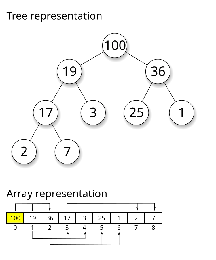
Heap sort

Heap sort is also an efficient $O (n \log n)$ sorting algorithm. However, inside the heap, the elements are not fully sorted. For example, below is a max-heap tree, and we are currently building the tree (inserting numbers to the heap one by one). Suppose we insert a new node (24) to the tree, by convention as a child node of (3). Then we sift up the new node, swapping with (3) then with (19). After 2 swaps, the node is settled. But how many new inversions does this insertion contribute to? It must be more than 2, since before this insertion, there are already 3 numbers that are smaller than 24, namely 25, 36, and 100. Therefore, the actual inversions are (25, 24), (36, 24), and (100, 24), which have nothing to do with the two sift-ups.

Source: https://en.wikipedia.org/wiki/Heap_(data_structure) (CC BY-SA 4.0)

Source: Heap (data structure) - Wikipedia (CC BY-SA 4.0)

In general, when we are inserting nodes into the heap, only the “maximum/minimum” are maintained, while both the indices and the inequality relations are lost. Even if we kind of store them somewhere (like inside the nodes), it is hard to infer the inversion numbers from the sift-ups. Therefore, we can’t use heap sort to calculate the inversion number.

Mission failure!

Counting sort

Here comes the interesting part. Counting sort is definitely a time-optimal algorithm (though space consuming), so why not try to use it to solve the problem?

And the how-to is already within our hands — when we are analyzing the heap sort (and insertion sort), we found that we just have to count how many previously inserted elements are greater than it. This leads to a pretty straightforward algorithm:

def counting_sort(A: list[int]):
    count = 0
    buckets = [0] * (max(A) + 1)
    buckets[A[0]] += 1
    for i in range(1, len(A)):  # current element to insert
        buckets[A[i]] += 1
        for j in range(A[i] + 1, len(buckets)):
            count += buckets[j]  # every already-inserted element greater than A[i]
    return count

Woohoo, an $O (n m)$ algorithm! (Let $m$ be $max {A_{i}}$ .)

But do we really need that many buckets?

Discretization. We could reduce the needed buckets by sorting beforehand 😆 (not sarcasm). Suppose we have a sequence of (20, 40, 30, 70, 50). Naturally we want to reduce it down to (2, 4, 3, 7, 5), or even (1, 3, 2, 5, 4). The latter is called the “discretized sequence.”

def discretize(A: list[int]):
    # Add indices to the list
    A = [(i, x) for i, x in enumerate(A)]

    # Sort by values then indices (stable sort)
    A = sorted(A, key=lambda x: (x[1], x[0]))

    # Add new indices (discretized values) to the list
    A = [(j, i, x) for j, (i, x) in enumerate(A)]

    # Sort by original indices
    A = sorted(A, key=lambda x: x[1])

    # Return only the discretized values (1-based indexing)
    return [j + 1 for j, i, x in A]

By discretization, we can reduce the number of buckets down to $n$ , and therefore, reduce the time complexity down to $O (n^{2})$ .

But that’s not what we came here for! We want a more optimal algorithm, at least as efficient as $O (n \log n)$ .

Luckily, there are data structures that can achieve $O (\log n)$ for calculating “how many elements previously inserted are greater than it.” Don’t scroll down — can you think of any?

Here are two data structure examples that can efficiently maintain interval sum dynamically.

(1) Segment tree

A segment tree is similar to a binary search tree — it divides the interval into halves, quarters, and so on. Each leaf node is the smallest undividable unit of the interval.

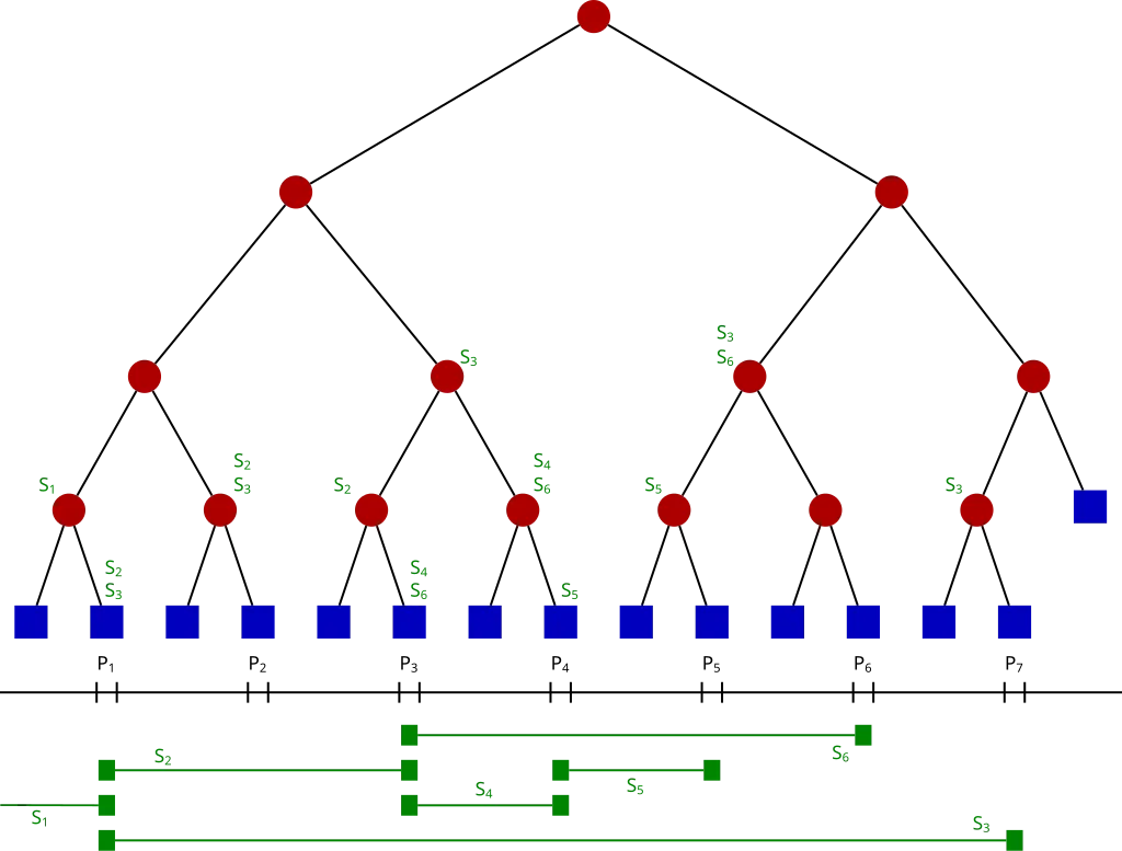
Source: https://en.wikipedia.org/wiki/Segment_tree (CC BY-SA 4.0)

Source: Segment tree - Wikipedia (CC BY-SA 4.0)

For our problem, we want to calculate the number of $A_{j}$ greater than $A_{i}$ but inserted before it ( $j < i$ ). Therefore, we can build a segment tree of interval $[0, m]$ . Then we insert all elements one by one, and query the segment tree to get the occurrence counts.

class SegmentTree:
    def __init__(self, n: int):
        self.n = n
        self.tree = [0] * (4 * n)  # 1-based indexing

    def add(self, i: int, value: int):
        def add_recursive(node: int, left: int, right: int):
            if left == right:
                self.tree[node] += value
                return

            mid = (left + right) // 2
            if i <= mid:
                add_recursive(node * 2, left, mid)
            else:
                add_recursive(node * 2 + 1, mid + 1, right)
            self.tree[node] = self.tree[node * 2] + self.tree[node * 2 + 1]

        add_recursive(1, 1, self.n)

    def query(self, l: int, r: int):
        def query_recursive(node: int, left: int, right: int):
            if l > right or r < left:
                return 0
            if l <= left and r >= right:
                return self.tree[node]

            mid = (left + right) // 2
            l_sum = query_recursive(node * 2, left, mid)
            r_sum = query_recursive(node * 2 + 1, mid + 1, right)
            return l_sum + r_sum

        return query_recursive(1, 1, self.n)

def counting_sort_segment_tree(A: list[int]):
    count = 0
    # A = discretize(A)  # if you wish to apply discretization
    segment_tree = SegmentTree(max(A))
    segment_tree.add(A[0], 1)
    for i in range(1, len(A)):  # current element to insert
        count += segment_tree.query(A[i] + 1, max(A))
        segment_tree.add(A[i], 1)
    return count

When not discretized, the runtime complexity is $O (n \log m)$ , while the space complexity could reach up to a crazy $O (m)$ . When discretized, the runtime complexity reduces to $O (n \log n)$ .

(2) Fenwick tree

I hope you’ve heard of the Fenwick tree, or binary indexed tree (BIT). If not, you could refer to the following diagram:

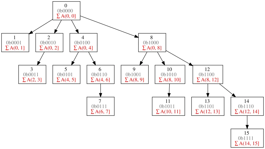
Source: https://en.wikipedia.org/wiki/Fenwick_tree (CC BY-SA 4.0)

Source: Fenwick tree - Wikipedia (CC BY-SA 4.0)

—It’s basically a prefix sum, isn’t it?

If we store the occurrence counts in a Fenwick tree, we could infer the new inversions when inserting $A_{i}$ by calculating $i - prefix sum (A_{i})$ . Why? Because $prefix sum (A_{i})$ is the previous occurrences of elements that are not greater than $A_{i}$ , and there are $i$ elements currently considered, then $i - prefix sum (A_{i})$ must be the previous occurrences that are greater than $A_{i}$ .

class FenwickTree:
    def __init__(self, n: int):
        self.n = n
        self.tree = [0] * (n + 1)  # 1-based indexing

    def add(self, i: int, value: int):
        while i <= self.n:
            self.tree[i] += value
            i += i & -i

    def query(self, i: int):
        prefix_sum = 0
        while i > 0:
            prefix_sum += self.tree[i]
            i -= i & -i
        return prefix_sum

def counting_sort_fenwick_tree(A: list[int]):
    count = 0
    # A = discretize(A)  # if you wish to apply discretization
    fenwick_tree = FenwickTree(max(A))
    fenwick_tree.add(A[0], 1)
    for i in range(1, len(A)):  # current element to insert
        count += i - fenwick_tree.query(A[i])
        fenwick_tree.add(A[i], 1)
    return count

Similar to the segment tree implementation, when not discretized, the runtime complexity is $O (n \log m)$ , and when discretized, the runtime complexity reduces to $O (n \log n)$ .

#Algorithms